I have been writing about polygyny for years now. The main thrust of my argument has been that high rates of polygyny commonly involve relatively coercive, male-biased marriage arrangements, and that rather than polygyny being sustained by women seeking to share a wealthy man, it is often men who use these arrangements to appropriate women’s surplus labor and benefit themselves (read the links above for examples). I’m not saying this is always the case, just that it is a common pattern, and a particularly salient one when the percentage of polygynous marriages within a society is high.
My arguments have been based on my read of the ethnohistorical evidence, however I have not formally tested these ideas. Here I provide a brief reanalysis of Marlowe (2003) and make some predictions which I will test further with a larger dataset (Binford, 2001) in Part 2.
In his 2003 paper Frank Marlowe investigated patterns of polygyny among the hunter-gatherer societies in the Standard Cross-Cultural Sample (n=36). Marlowe used the existing SCCS codes for his analysis, and also helpfully provided some of the data he used in that paper. I have taken the data from his paper as well as the SCCS codes available on D-PLACE to replicate his work. There are two key patterns he found which I want to discuss here.
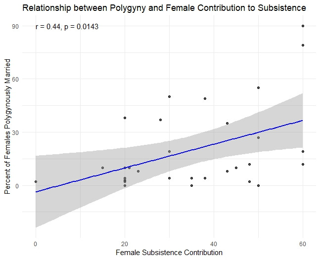
First, Marlowe found a significant negative relationship between mean male contribution to subsistence and the percent of married women who are polygynously married (r = -.44, p = 0.014, n = 30). Since my emphasis here is on female subsistence I used mean female contribution instead. Marlowe actually used the EA code for female contribution to subsistence and subtracted it from 100, so I am essentially just using the original variable. I found the exact same result that he did (positive rather than negative though, obviously, since I’m using female contribution rather than male).
Note that many of the graphs I made below say something like “Percent of Females Polygynously Married” but should instead say something like “Percent of Married Females Who Are Polygynously Married” to more accurately reflect the code, as the code only includes those who already married rather than all females more generally as my graphs might erroneously imply (I use the term female rather than women because many of those already married may still be very young girls, while women implies adults). I regret the imprecision, but I’m not going to redo all the graphs, so just keep that in mind.
Ethnographic descriptions from societies within our dataset describe the pattern well. Among the Shavante of Brazil, where 49% of married women are polygynously married according the SCCS code, Maybury-Lewis (1967) notes that, "wives are an economic asset,” and discusses Lévi-Strauss’ work among the nearby Nambikwara, where “A man with a number of wives could acquire a food surplus which enabled him to be generous to others, or alternatively to devote his time to matters of public concern rather than to the domestic business of providing for his family.”
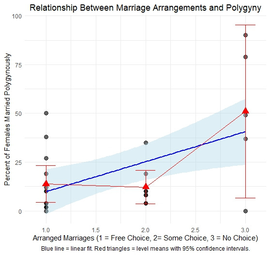
Next, Marlowe found a significant positive correlation between arranged marriage of females and percent of married women polygynously married (r = 0.502, p = 0.009, n = 26). The SCCS arranged marriage scale is an ordinal variable with six levels which Marlowe transformed into three. I think this was legitimate since the original variable makes various more subtle distinctions which are not especially relevant here, while Marlowe simplifies it so, “1 = individual selects or parental approval highly desirable; 2 = individual suggests partner and then others arrange, individual choice or arrangement are alternatives, or parents choose but individual can object; 3 = parents choose, individual cannot reject.”
Essentially, 1 is complete or nearly complete free choice, 2 is some choice, and 3 is no choice.
Marlowe treats the variable as continuous, which I also do here, and again I find the exact same result (r = 0.502, p = 0.009, n = 26). To better visualize the relationship I plotted it with a linear fit and the level means included below:
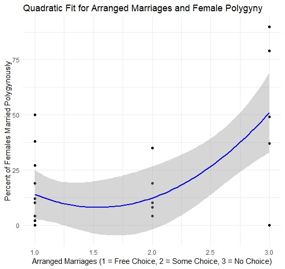
Obviously there is an important nonlinear relationship here, another way of showing it is visualizing the fit from a quadratic model:
As you can see the most salient category is level 3, where females have no choice in marriage arrangements. Where there is full choice or some choice you aren’t generally seeing a lot of polygyny, but where there is no choice at all you have the highest rates. Note there is one outlier in the no choice category at 0% which—along with the small sample size—is driving the wide confidence interval. That is the Vedda of Sri Lanka. Notably their female subsistence contribution is coded in the SCCS as only 20%, so despite their stringent marriage arrangements their lack of polygyny is not entirely unexpected considering the important role of female subsistence contribution, as I will discuss further towards the end of this post.
You may also notice the 50% outlier in the free choice category, which I suspect is a flawed code. That society is the Aweikoma of Brazil, and based on the sources provided on D-PLACE to support the codes (Jungle People: a Kaingang tribe of the highlands of Brazil, Henry 1964 and The Caingang, Metraux 1946) I think the percent of polygynous marriages may be incorrect and the arranged marriage code should be at least a 2.
According to the SCCS codes 30% of married males and 50% of married females are married polygynously, although I’m not sure where those figures come from exactly. I may have missed it, but the only numbers I could find on polygyny are not directly comparable. Henry (1964) notes that “An analysis of 308 marriages taken from genealogies that represent about 100 years of Kaingáng history past and present, yields the following percentages: 60 percent monogamous, 18 percent polygynous, 14 percent polyandrous and 8 percent joint.” He does not give more information on sex. I suspect the issue of polyandry and “joint” marriages may have confounded the polygyny variable in some way.
Further, there appears to be less total free choice involved than the arranged marriage variable implies. Metraux (1946) discusses child betrothals:
According to Baldus' census (1937 c, p. 43), men are generally older than their wives, in some cases as much as 15 to 20 years; among 37 percent of the couples there was a difference of 10 years. A man marries when 18 to 20 years of age. If his bride is not yet of age, he stays with her parents, waiting for the first signs of puberty. In case of child betrothal, the lad's parents have to provide for the girl's subsistence.
And he further notes one such case of an apparently very coercive arranged marriage,
A marriage ceremony witnessed by Manizer (1930, p. 776) took place during a drinking bout. Some old men seized the bridegroom and bride and pushed them toward each other in spite of the woman's resistance. Then they dragged them into the bridegroom's hut and left them there under a blanket. The following day the woman ran away, but was brought back by force.
I may go through many of these codes in more detail in a future post to evaluate their accuracy, but here I’m mostly just going to stick with what we’ve got.
A key point raised by the ethnographic example of the Aweikoma noted above is the importance of age in relation to both arranged marriages and polygyny. Since young girls are generally going to have less social power and/or ability to exercise choice than adult women, you would expect arranged marriages to be more coercive and more oriented towards polygyny among them.
Among the Yolngu of Australia high rates of polygyny are enabled by infant bestowal, "Put simply, Yolngu men and women spoke of a woman being 'given' to a man rather than the other way round. Many marriages were arranged when the prospective husband was young, and even before the birth of the girl who would be the wife." (Keen, 1994). And many women may unsurprisingly not prefer these kind of arrangements. Keen (1994) cites Janice Reid’s work interviewing Yirrkala women of Australia, where despite a history of normative polygyny, women prefer monogamy, at least in more recent years, “The preference for monogamous marriages is now quite strong, at least among women. When I asked 41 women of the community how many wives a man should have, 32 said one and nine said two or more.” (Reid, 1983).
Among the Shavante, marriages are arranged when the girls in particular are very young and have little say in the matter,
The arrangements are made initially by the parents of the parties concerned...Since the prospective bride and bridegroom are so young, their wishes are not usually taken into consideration. The girls are frequently too small to understand the negotiations anyway. The boys, on the other hand, may manage to have their preferences considered by their elders (Maybury-Lewis, 1967).
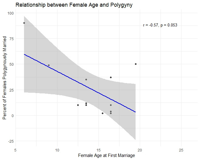
I wanted to test if there’s a relationship between female age at first marriage and the percent of married females married polygynyously, so I got the SCCS codes from D-PLACE on age at first marriage and compared them to the polygyny data provided by Marlowe. Unfortunately there is a lot of missing data, so we only have 12 societies with data on age at first marriage and polygyny, however we do see the predicted pattern (r = -0.57, p = 0.053).
Obviously that p value isn’t very compelling, but with n = 12 that is to be expected, and we do see a moderate effect, with polygynous marriages being more common where age at first marriage for females is younger. Notably that 50% outlier is the Aweikoma again—according the SCCS codes the age at first marriage for females is 19.5! This is obviously wrong in light of what Metraux said above, so even this moderate relationship we found may undersell things. Because of the small sample size I can’t do much more with this, but when I make use of the Binford dataset in Part 2 I’ll look into the impact of age on polygyny.
Playing around with the Marlowe data further, I performed a multiple linear regression assessing the impact of arranged marriages and female subsistence contribution on polygyny:
I standardized the coefficients (β) for ease of comparison because we’re working with variables on different scales (female subsistence contribution is a percentage and arranged marriage is a three-point scale). As you can see in the table above the model has a moderate effect size (R² = .37) and both predictors remain individually significant when holding the other constant.
Of course, as the plots I posted further above indicated, there is a nonlinear relationship between our arranged marriage scale and the percent of married females married polygynously, so I also performed an explicit quadratic regression model:
This is a stronger model and captures that the main impact of arranged marriages on polygyny is coming from no choice rather than a linear trend. Since the quadratic term is capturing most of the variance in the relationship between polygyny and arranged marriages it’s not surprising the linear term is nonsignificant, as they overlap.
Now one very important point, which I haven’t raised until now, is the issue of Galton’s problem. Societies that are more closely related to each other historically or that have interacted with each other previously often share beliefs and practices that don’t reflect independent origins, meaning treating societies as independent datapoints poses some difficulties, confounding the correlations and models I described above. It could be that these patterns reflect a shared cultural history of societies in particular regions rather than independent causal effects.
D-PLACE has latitude and longitude data for each society, and I also made use of this language phylogeny, to measure spatial autocorrelation (Moran’s I) and the phylogenetic signal (Blomberg’s K) for the three key variables I’ve been discussing:
The results indicate that the percent of females married polygynously and female subsistence contribution each exhibit moderate phylogenetic signal and evidence of spatial autocorrelation. That is, societies that are more closely related to each other (as measured by their position in the language phylogeny) and closer to each other spatially, have more similar rates of polygyny and mean female contribution to subsistence. Arranged marriages however don’t show a significant phylogenetic signal or evidence of spatial autocorrelation.
The Standard Cross-Cultural Sample was created specifically to try and account for Galton’s problem by pruning the Ethnographic Atlas and sampling only 1 society each from 186 different culture areas, but it is imperfect, particularly in this case where we’ve cut down the sample to only the hunter-gatherers in it.
I performed a phylogenetically controlled regression using Brownian Motion to model trait evolution, which can help account for cultural relatedness (but not spatial autocorrelation directly), and we get very similar results, although the coefficients are a bit smaller, and there is still evidence of residual phylogenetic signal that our model isn’t capturing (K = 1.06, p = 0.018).
One problem with the above is the regression methods I used assume a normal distribution for the response variable (female polygyny) but rates of female polygyny are not normally distributed across societies (W = 0.78, p < 0.001), so I also performed a beta regression as they’re good for modeling proportional data. Since beta regressions require values to be strictly between 0 and 1, I rescaled and adjusted the boundary values of the female polygyny variable (y(n−1) + 0.5/n). Because the values in our polygyny variable are skewed near 0 (as you can see from the plots above) I performed the arcsine square root transformation to handle the skew. We see very similar results here, although female subsistence contribution is no longer significant (p = 0.06), perhaps due in part to our small sample size. Keep in mind the coefficients here are not directly comparable to the other models because of the arcsine transformation:
Another way of testing these relationships is through a generalized additive model (GAM) with a spatial smoothing term s(Latitude + Longitude), which can help account for spatial autocorrelation (but not cultural relatedness directly).) I used the complementary log-log function in R for this beta model to handle the skew of female polygyny:
Another similar result here, although again female subsistence contribution is not significant, which is plausibly due both to our small sample size but also because female contribution covaries with latitude (r = -0.47, p = 0.015), so attempting to account for spatial autocorrelation in this somewhat crude fashion might suppress some of this effect.
Additionally, neither the phylogenetic regression nor the GAM can account for both phylogenetic influence and spatial autocorrelation together.
Finally, I wanted to perform a Bayesian model that could help account for both phylogenetic and spatial patterns. I performed a Bayesian beta regression with phylogenetic and spatial random effects using weakly informative priors. I used a phylogenetic variance-covariance matrix derived from the tree, and a spatial correlation matrix based on geographic distance between societies using exponential decay. I plotted the posterior probability distribution below:
Overall the effect of arranged marriages (β̃ = 0.35, pd = 0.94) and female subsistence contribution (β̃ = 0.38, pd = 0.94) on polygyny does seem pretty robust even when incorporating phylogenetic and spatial controls. There was evidence of both phylogenetic (SD = 0.41, 90% HPDI [0.0003, 1.04]) and spatial (SD = 0.74, 90% HPDI [0.005, 1.41]) effects in the model, although a lot of uncertainty as you can see, due to our small sample size. [Note: “the probability of direction (pd) [is] the proportion of the posterior distribution that is of the median's sign (i.e. greater or less than 0) (Makowski, Ben-Shachar and Lüdecke 2019; McElreath 2020). We interpret associations between predictors and outcomes as strong evidence when 90% of posterior distributions do not include 0 and as moderate when 80% of posterior distributions do not include 0.” (Garfield et al, 2023)]
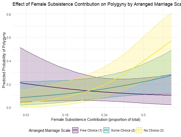
We can also model the impact arranged marriages and female subsistence contribution have on polygyny as an interaction effect in a Bayesian beta regression, and I found a very strong result (β̃ = 0.62, pd = 0.96). I plotted the model predictions below, which I think does a good job of illustrating the pattern. The model has good predictive accuracy, as the predicted polygyny rates from the model are strongly correlated with the actual rates (r = 0.951, MAE = 0.068).
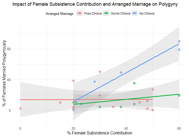
Notably it seems to be the combination of high female contribution to subsistence and coercive arranged marriages interacting together that most strongly promote high rates of polygyny.
As another check I also calculated the relationship between female subsistence contribution and percent of females married polygynously for each arranged marriage level: for societies with free choice there was essentially no relationship between female subsistence contribution and polygyny (r = 0.007, p = 0.98, n = 13), with some choice there was a small positive but non-significant relationship (r = 0.45, p = 0.27, n = 8), and for societies with no choice there was a significant positive relationship (r = 0.97, p = 0.007, n = 5). Here’s how they look plotted as linear relationships:
Of course these are small sample sizes and the simple correlations don’t control for phylogeny or spatial autocorrelation so the Bayesian model was worth doing, but it’s nice that we’re seeing the same thing across different ways of handling the data.
Conclusion
I think these results make a lot of sense. If arranged marriages are coercive, but males still contribute most of the subsistence, high rates of polygyny generally cannot be maintained because most males can’t support multiple wives. Conversely, if marriages are grounded in free choice, but females contribute most of the subsistence, high rates of polygyny may be difficult to maintain because most women would likely prefer not to have to share a partner. But when females contribute most of the subsistence, arranged marriages are highly coercive, and (I hypothesize) female marriages are arranged at a very young age, it is much easier to sustain higher rates of polygyny.
Overall I think these results are suggestive and a useful replication of Marlowe’s work, but we are still hampered by the small sample size and coarse measures. In Part 2 I will make use of the Binford hunter-gatherer dataset, which is much larger, and in Part 3 I will delve into the ethnographic sources for the individual codes to see how well they hold up.
For two great related papers see Ross et al (2018) - Greater wealth inequality, less polygyny: rethinking the polygyny threshold model and Minocher et al (2019) - Explaining marriage patterns in a globally representative sample through socio-ecology and population history: A Bayesian phylogenetic analysis using a new supertree.
The Ross paper effectively explores some of the important socioecological dynamics related to male wealth and polygyny, although they use a mutual mate choice model, which is very different from the perspective I take here.
The Minocher paper is quite compatible with my results—they found a solid probability of direction for arranged marriages predicting the percent of married men who are polygynous across the entire SCCS (pd = 0.94), which is exactly what I found looking at the impact of arranged marriages on the percent of females married polygynously in my Bayesian model (pd = 0.94). They also found a strong probability of direction for female agriculture on the percent of married men who are polygynous (pd = 0.96) which is close to what I found for the effect of female contribution to subsistence on the percent of married women married polygynously (pd = 0.94). I used a different phylogenetic tree and just looked at the hunter-gatherers in the SCCS so the similar results are encouraging I think.





Welcome back
Interesting. I've been toying around with the idea that there are two different kinds of polygyny, let's call them "lion polygyny" and "sultan polygyny".
In lion polygyny the females contribute most of the resources and the male spends his time defending his harem against other males. In sultan polygyny the male contributes most of the resources. Notice that sultan polygyny requires the man to be able to contribute more resources than all his wives combined could do on their own. Since humans aren't that sexually dimorphic, this is only possible if the man in question sits at or near the top of a massive power structure. This is probably also why there don't appear to be any examples of sultan polygyny in the animal kingdom.